Geoexamples - Cloud Optimized GeoTIFF tutorial

Cloud Optimized GeoTIFF (COG) is simply an intelligent way to store a GeoTIFF file. Or, better defined in the COG web site:

A Cloud Optimized GeoTIFF (COG) is a regular GeoTIFF file, aimed at being hosted on a HTTP file server, with an internal organization that enables more efficient workflows on the cloud. It does this by leveraging the ability of clients issuing HTTP GET range requests to ask for just the parts of a file they need.

In this short tutorial, you can find how to create them, and how to read them from a browser or the command line.

The Cloud Optimized Geotiff format
Creating a Cloud Optimized GeoTIFF
Reading a Cloud Optimized GeoTIFF file
- Using geotiff.js to read a COG
  - An example with RGB
  - An example with numerical data
- Using GDAL to read a COG
Links

The Cloud Optimized Geotiff format

Cloud Optimized GeoTIFFs, as explained in the previous section, are organized to be downloaded by parts. When a file os properly organized, the HTTP GET range request (“bytes: start_offset-end_offset” HTTP header) can be used, and only the parts needed are downloaded.

As Even Rouault explains in the GDAL COG page, the structure is:

TIFF / BigTIFF signature
IFD (Image File Directory) of full resolution image Values of TIFF tags that don’t fit inline in the IFD directory, such as TileOffsets?, TileByteCounts? and GeoTIFF keys
Optional: IFD (Image File Directory) of first overview (typically subsampled by a factor of 2), followed by the values of its tags that don’t fit inline
Optional: IFD (Image File Directory) of second overview (typically subsampled by a factor of 4), followed by the values of its tags that don’t fit inline
…
Optional: IFD (Image File Directory) of last overview (typically subsampled by a factor of 2N), followed by the values of its tags that don’t fit inline
Optional: tile content of last overview level
…
Optional: tile content of first overview level
Tile content of full resolution image.

There are two important parameters to set which aren’t in the standard

The tile size. Usually is 256x256 or 512x512 pixels
The compression type. LZW is accepted more easily than DEFLATE, but the later compresses more

Creating a Cloud Optimized GeoTIFF

The easiest way to create a COG is using the GDAL command line interface. If the GeoTIFF data is created from a script using GDAL, it is also possible to do it inside using python or any language with the GDAL bindings.

But, before trying to convert anything, better check if the file is already in a good format and if you prefer using overviews or not.

Create a COG using GDAL from the command line

The basic thing to understand is that the GeoTIFF must be tiled. This is, that instead of writing all the row, the image is divided in small tiles, so only some of them are downloaded. Compression can be DEFLATE or LZW. The first compresses more but is less compatible with some libraries.

$ gdal_translate ori.tiff out.tiff -co COMPRESS=LZW -co TILED=YES

This is ok if you want to download all the bands at once, like in an aerial photo. If you have independent bands, or many of them, you may want to download only one band at once. The, you may use the INTERLEAVE=BAND option:

$ gdal_translate ori.tiff out.tiff -co COMPRESS=LZW -co TILED=YES -co INTERLEAVE=BAND

Overviews

The TIFF format allows to store more than one image, the same way a PDF can store more than one page. This can be used to create the overviews or pyramids. Each overview will divide the image in four from the previous level, so a smaller amount of data can be read. In our case, a thumbnail of a huge GeoTIFF could be easily shown without reading all the pixels.

This is independent of the tiling part, but combining both allows to make efficient files for reading a small part of the image and for zooming out efficiently at the same time.

GDAL has a cli command to create the pyramids called gdaladdo. The command must be run BEFORE the gdal_translate or the resulting GeoTIFF won’t be COG compliant.

This would make four overview images by averaging the values:

$ gdaladdo -r average abc.tif 2 4 8 16

Create a COG using gdal-python

The previous section results can be achieved using python directly, which is nice to integrate in the scripts that generate data.


import gdal
import numpy as np

x_size = 10000
y_size = 10000
num_bands = 4
file_name = "/tmp/test.tiff"

data = np.ones((num_bands, y_size, x_size))
driver = gdal.GetDriverByName('GTiff')
data_set = driver.Create(file_name, x_size, y_size, num_bands,
gdal.GDT_Float32,
options=["TILED=YES",
"COMPRESS=LZW",
"INTERLEAVE=BAND"])

for i in range(num_bands):
data_set.GetRasterBand(i + 1).WriteArray(data[i])

data_set.BuildOverviews("NEAREST", [2, 4, 8, 16, 32, 64])
data_set = None

As you can see, the creation options are passed as a parameter when creating the data set
Also, the gdal-python bindings have a nice method to create the overviews. The problem is that this will give an error in the COG format, because the pyramids were created after the tiling. It’s not a big error, as we will see in the next section, but you can avoid it by using a memory driver file before creating the actual one:


import gdal
import numpy as np

x_size = 10000
y_size = 10000
num_bands = 4
file_name = "/tmp/test.tiff"

data = np.ones((num_bands, y_size, x_size))
driver = gdal.GetDriverByName('MEM')
data_set = driver.Create('', x_size, y_size, num_bands,
gdal.GDT_Float32)

for i in range(num_bands):
data_set.GetRasterBand(i + 1).WriteArray(data[i])

data = None
data_set.BuildOverviews("NEAREST", [2, 4, 8, 16, 32, 64])

driver = gdal.GetDriverByName('GTiff')
data_set2 = driver.CreateCopy(file_name, data_set,
options=["COPY_SRC_OVERVIEWS=YES",
"TILED=YES",
"COMPRESS=LZW"])
data_set = None
data_set2 = None

Checking if a GeoTIFF is a valid COG

Even Rouault made a nice python script that not only checks if the file is a correct COG, but also gives some tips to improve the ones that are correct.

For instance, the file in the ObservableHQ example works, but it’s a not valid COG, because of a problem with the overviews. The script output is:


$ python3 validate_cloud_optimized_geotiff.py SkySat_Freeport_s03_20170831T162740Z3.tif

SkySat_Freeport_s03_20170831T162740Z3.tif is NOT a valid cloud optimized GeoTIFF.
The following errors were found:

- The offset of the first block of overview of index 3 should be after the one of the overview of index 4
- The offset of the first block of overview of index 2 should be after the one of the overview of index 3
- The offset of the first block of overview of index 1 should be after the one of the overview of index 2
- The offset of the first block of overview of index 0 should be after the one of the overview of index 1
- The offset of the first block of the main resolution image should be after the one of the overview of index 4


We can easily correct it by running:

  gdal_translate SkySat_Freeport_s03_20170831T162740Z3.tif correct_SkySat_Freeport.tiff -co COMPRESS=LZW -co TILED=YES

Now, the output gives a warning, instead of an error:

```bash
$ python3 validate_cloud_optimized_geotiff.py correct_SkySat_Freeport.tif

The following warnings were found:

- The file is greater than 512xH or Wx512, it is recommended to include internal overviews


So the previous part removed the internal overviews. That's because we didn't use the _-co COPY_SRC_OVERVIEWS=YES_ option:

  gdal_translate SkySat_Freeport_s03_20170831T162740Z3.tif correct_SkySat_Freeport.tiff -co COPY_SRC_OVERVIEWS=YES -co COMPRESS=LZW -co TILED=YES

It's important to create the overviews _before_ transforming the file into a GeoTIFF, or otherwise the order will be wrong and the test won't pass. It will probably work anyway, but it's better to go with the specification. There's [a post by Even Rouault][cog_overviews_error] with a discussion about this error.

## Reading a Cloud Optimized GeoTIFF file

COG can be used to store a huge multi-layer file in the cloud so your scripts can use parts of it, or you can download the part you need to create an interactive map, or use [Terracotta][terracotta] to create the tiles directly at AWS uploading only the whole GaoTIFF.

### Using geotiff.js to read a COG

The awesome geotiff.js has been adapted to read COG files, which make really easy to use them without thinking about the format.

I learnt how to work with COG and geotiff.js looking at [this ObservableHQ example][observable_example]. I'll try to expand a little the important points.

The first point to understand is that geotiff-js has now many asynchronous methods, because it has to open the file, but also read the different parts of it. Let's see a small example that just reads a square of 10x10 pixels.

```js
(async function () {
const tiff = await GeoTIFF.fromUrl("out.tiff");
console.log("Number of images (pyramids):", await tiff.getImageCount());

const image = await tiff.getImage();
console.log("Bounding box:", image.getBoundingBox());
console.log("Width:", image.getWidth());

let data = await image.readRasters({
  window: [200, 200, 210, 210],
  samples: [0],
});

console.log("Values:", data);
})();

The output is:

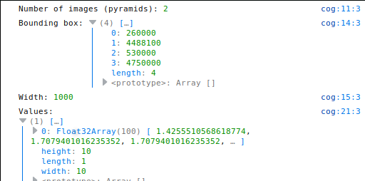
I used the async/await technique to make the code easier to understand. In this case, opening the image, getting the actual image and reading the image data are three asynchronous methods.
getImage() will return the main pyramid, with the original resolution. Is the same as .getImage(0). In the example, another pyramid is created, so using .getImage(1), an image with a 500px width would returned
The image object has all the pyramid properties, but not the actual data, which has to be retrieved using the readRasters method
- The readRasters method has several options. In this case, the window argument asks to get only some of the pixels, taking advantage of being a COG
- The samples parameter is the band number. The example file had two separate bands, so using samples: [1] would return the second band. All the desired bands can be passed into this parameter, so the result of samples: [0, 1] would be an array with two Float32Array elements, one for each band

What about the queries? This is the network tab on the developer tools:

We can see three downloads of the out.tiff file:

The first one is the header for the main image.
The second the header for the first pyramid. If the image had no pyramids, this wouldn’t appear.
The third is the data (note the different size).
- If two different bands are to be retrieved, an extra request will appear. This is because I separated the tiff in separate bands, since they are data bands. If the file is a satellite with the rgb bands, keeping the three bands together would be more efficient.

Note that all the above has been transparent, which is really cool.

An example with RGB

There’s a nice example at ObservableHQ showing how to use an RGB GeoTIFF when it’s cloud optimized.

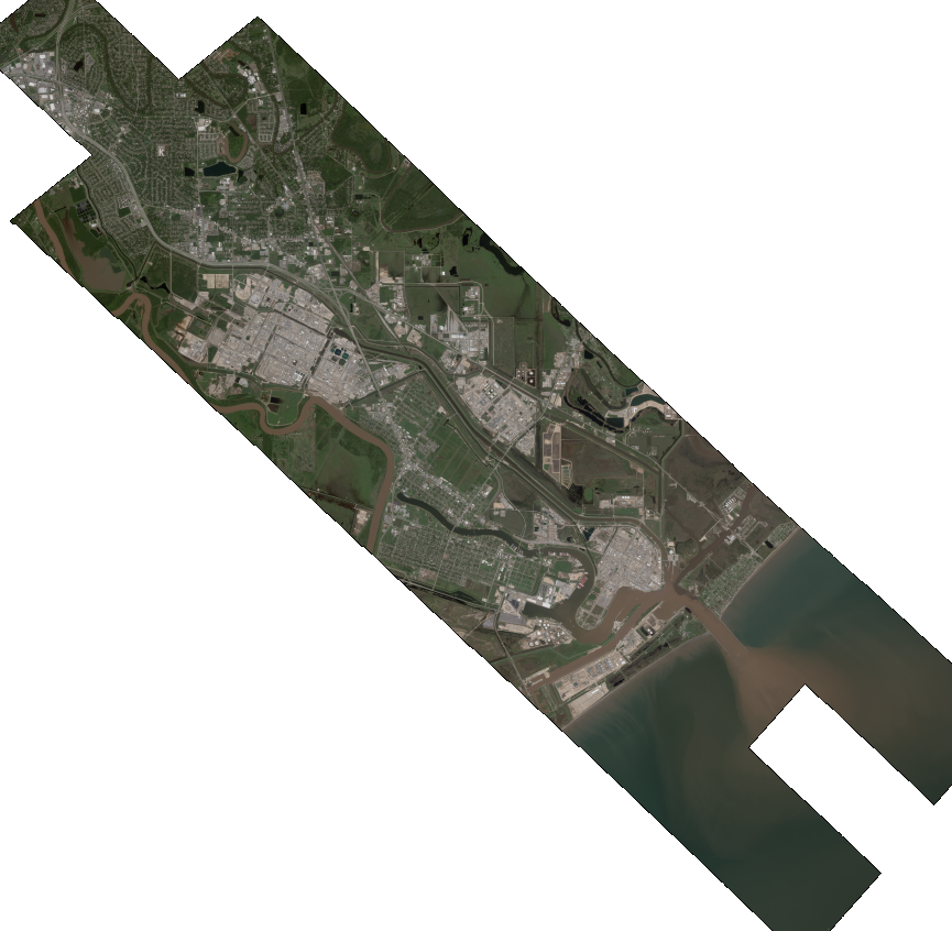
The interesting part is this one:


readImageData = async (image, options = {}) => {
const rasters = await image.readRasters(options);
let [r, g, b] = rasters;
let { width, height } = rasters;
const data = new Uint8ClampedArray(width _ height _ 4);
for (let i = 0; i < r.length; i++) {
data[i * 4] = r[i];
data[i * 4 + 1] = g[i];
data[i * 4 + 2] = b[i];
data[i * 4 + 3] = r[i] == 0 ? 0 : 255;
}
return new ImageData(data, width, height);
}

The r,g and b channels are separated in layers, but to draw the image, we want it in a Uint8ClampedArray
context.putImageData(data, 0, 0); is then the way to draw the data directly. Quite easy!

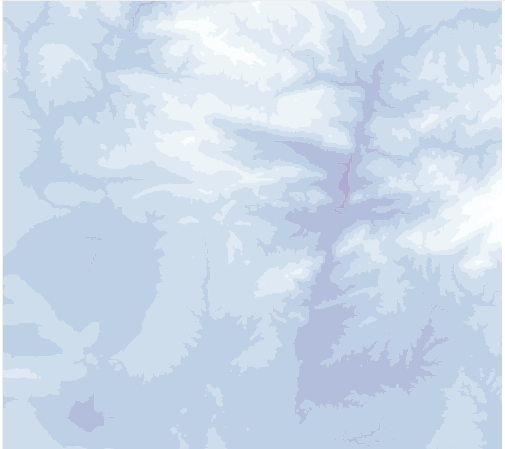
An example with numerical data

In this case, the data in the GeoTIFF is a matrix with the numerical values (temperature in our case). The sample.tiff file is big, 26MB, so making the client to download all the data is not an option.

I’m using the marching squares algorithm to show the regions where the data is between two thresholds. You can see a tutorial here.

Click here to see the working example]

(async function () {
  const tiff = await GeoTIFF.fromUrl("sample.tiff");
  let image = await tiff.getImage(3);
  let rasterData = await image.readRasters({ samples: [0] });
  rasterData = rasterData[0];

  let data = new Array(image.getHeight());
  for (let j = 0; j < image.getHeight(); j++) {
    data[j] = new Array(image.getWidth());
    for (let i = 0; i < image.getWidth(); i++) {
      data[j][i] = rasterData[i + j * image.getWidth()];
    }
  }

  let intervals = [-2, 0, 2, 4, 6, 8, 10, 12, 14, 16, 18, 20];
  let bands = rastertools.isobands(data, [0, 1, 0, 0, 0, 1], intervals);

  let colorScale = d3.scaleSequential(d3.interpolateBuPu);
  let canvas = d3
    .select("body")
    .append("canvas")
    .attr("width", 680)
    .attr("height", 500);

  let context = canvas.node().getContext("2d");

  let path = d3.geoPath().context(context);

  bands.features.forEach(function (d, i) {
    context.beginPath();
    context.globalAlpha = 0.7;
    context.fillStyle = colorScale((2 + intervals[i]) / 22);
    path(d);
    context.fill();
  });
})();

The output will be like this (all the GeoTIFF coverage):

In this case, only the smallest overlay is used. Why? Because it’s got about 350x350 pixels. This is enough to create the isobands. So, in case you don’t know which overlay to take, this is a good orientation
- tiff.getImage(3) is the place where the overlay is chosen
The color scale and path drawing are using the usual d3js library tools. This is just an example and everything could be done with other tools, although d3js is still the best option

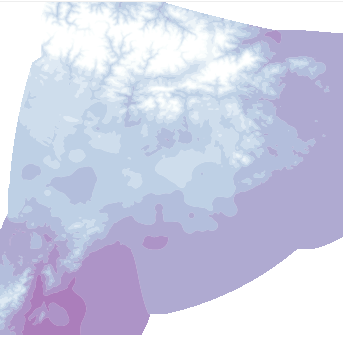
Let’s see another example using the image with the highest resolution, but downloading just a small part using the GeoTIFF capabilities.

Click here to see the working example]

(async function () {
  let origin = [700, 600];
  let size = [500, 450];
  const tiff = await GeoTIFF.fromUrl(
    "/rveciana/raw/9d9ef3282959a41c3e54cedb717bdddf/sample.tiff"
  );
  let image = await tiff.getImage(0);
  let rasterData = await image.readRasters({
    window: [origin[0], origin[1], origin[0] + size[0], origin[1] + size[1]],
    samples: [0],
  });
  rasterData = rasterData[0];

  let data = new Array(size[1]);
  for (let j = 0; j < size[1]; j++) {
    data[j] = new Array(size[0]);
    for (let i = 0; i < size[0]; i++) {
      data[j][i] = rasterData[i + j * size[0]];
    }
  }

  let intervals = [-2, 0, 2, 4, 6, 8, 10, 12, 14, 16, 18, 20];
  let bands = rastertools.isobands(data, [0, 1, 0, 0, 0, 1], intervals);

  let colorScale = d3.scaleSequential(d3.interpolateBuPu);

  let canvas = d3
    .select("body")
    .append("canvas")
    .attr("width", 680)
    .attr("height", 500);

  let context = canvas.node().getContext("2d");

  let path = d3.geoPath().context(context);

  bands.features.forEach(function (d, i) {
    context.beginPath();
    context.globalAlpha = 0.7;
    context.fillStyle = colorScale((2 + intervals[i]) / 22);
    path(d);
    context.fill();
  });
})();

The output will be like this (a zoomed portion of the previous example):

tiff.getImage(0) will get the main image, not an overview. Using tiff.getImage() would give the same result
Note that image.getHeight() and image.getWidth() have been changed by the width and height we want to show. That’s, of course, because we want to get just a part of the image
Now, the window parameter is used in image.readRasters, to select the portion we want to have. We set an offset (upper left pixel) and the size of the data we want
This case is a little slow because it has many pixels and generating the isobands takes a bit. An alternative could be using an overview or drawing the pixels directly, since they are small enough

Using GDAL to read a COG

A COG can be read from the command line too! This page explains how. It’s possible, for instance, to get a pixel value by using gdallocationinfo:

gdallocationinfo --debug on /vsicurl/http://even.rouault.free.fr/gtiff_test/S2A_MSIL1C_20170102T111442_N0204_R137_T30TXT_20170102T111441_TCI_cloudoptimized_512.tif  5000 5000

This will check the position 5000, 5000 on the defined file, which is located on a remote server. And will use the COG capabilities.

On the explanation page, it’s discussed that using overviews can be faster.

To read a part of the array and store it into a tiff file, use gdal_translate:

gdal_translate --debug on \
/vsicurl/http://even.rouault.free.fr/gtiff_test/S2A_MSIL1C_20170102T111442_N0204_R137_T30TXT_20170102T111441_TCI_cloudoptimized_512.tif \
-srcwin 1024 1024 256 256 out.tif

Again, this is discussed in the explanation page, comparing which type of file (with/without tiles or overviews) works better.

Table of Contents