Geoexamples - Complex GIS calculations with gpu.js: Temperature interpolation

The previous post I wrote showed how to use the gpu.js library for drawing maps with JavaScript after calculating the values with the user’s GPU.

While writting it, I was preparing this conference (in Spanish) for the 2018 edition of the “Jornadas SIG Libre” at Girona. The motivation of the talk was showing the possibilities of using the user’s GPU instead of the server to make complex GIS calculations on the fly, so the speed could be much higher and the use of the server almost negligible.

The example

Some years ago, I made a python script that calculates the temperature and relative humidity on a raster, taking as the initial data the weather stations available at the Catalan Meteorological Service. The resulting product is still in use, specially to detect if the current precipitation is in form of rain or snow. There are some papers about this too.

The idea is, then, calculating a temperature field with a good resolution taking as input the weather station data. The example has several steps with intensive calculations, so it’s a good study case for gpu.js.

The temperature depends on many things, but fits quite well this formula:

$$ temperature = \beta*{0} + \beta*{1} _ altitude + \beta_{2} _ distanceToCoast $$

So, given the station temperatures in a given moment and knowing the altitude and distance to the coast for each station, a multiple-linear regrssion can be done to get a formula.

To calculate the multipl-linear regression, the matricial formula is this one:

$$ \hat{\beta}=(X^{T}X)^{-1}X^{T}y\ \hat{y}=X\hat{\beta} $$

So there are matrix transpositions, matrix multiplications and other operations that are basic gpu.js examples. Anyway, this step uses only few values (we will be using about 180 weather stations), so I will use numeric.js that is still fast enough and simplifies the code.

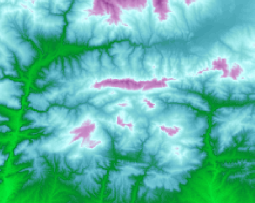
Once the beta values are calculated, a temperature field can be created if the altitude and distance values for each pixel are known. This is quite fast to do in gpu.js.

The result will look like this:

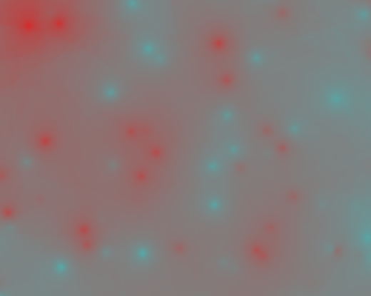
The problem with stopping here is that we are assuming that the formula is valid for all the territory, but we know that some regions have their own particularities (some regions may be a bit hotter or colder than what the formula expect). Let’s try to correct that with the residues method:

For each station, the real value is:

$$temperature = fit + residual$$

Using the matricial notation ,the errors or residuals are:

$$e=y-\hat{y}$$

Once we have the error in each point, we can interpolate them to create a residuals field that can be added to the original temperature calculation. To do it, we will use the inverse of the distance, which will give a result similar to:

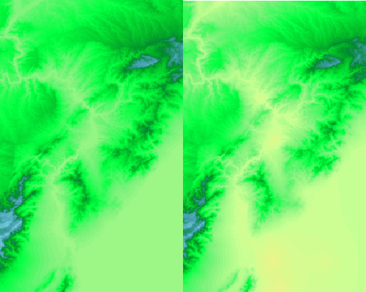
Finally, when adding the layer, some differences emerge:

So, to create the final map, the following things must be calculated. We will use a 1000x1000 pixels so the calculation is long using the CPU:

Calculation of the multiple linear regression
Creation of the temperature raster from the regression formula (GPU 1000x1000 px)
Residuals calculation
Residuals interpolation (GPU 1000x1000 px)
Final temperature field adding the temperature and residuals (GPU 1000x1000 px)
Layer representation (GPU 1000x1000 px)

The code

To make the example interactive and easier to split and understand, I made this observable notebook.

Multiple linear regression

I’m using numeric.js here to avoid many complex gpu.js coding, since with only two hundred weather station, the ellapsed time is a very small part of the total (2 ms).

let result = {};
const conv = convertData(data);
const X = conv.X;
const Y = conv.Y;
const X_T = numeric.transpose(X);
const multipliedXMatrix = numeric.dot(X_T, X);
const LeftSide = numeric.inv(multipliedXMatrix);
const RightSide = numeric.dot(X_T, Y);
result.beta = numeric.dot(LeftSide, RightSide);
const yhat = numeric.dot(X, result.beta);
result.residual = numeric.sub(Y, yhat);

Notice that the code is very easy to understand given the original formula:

$$ \hat{\beta}=(X^{T}X)^{-1}X^{T}y\ \hat{y}=X\hat{\beta} $$

Calculating the regression field

In this case, gpu.js will be used, since I’ve set a 1000x970 output field, which involves repeating the same operation about one million times, and this is where the gpu makes things much faster:


let gpu = new GPU();

const calculateInterp = gpu.createKernel(function(altitude, dist, regrCoefs) {
return regrCoefs[0] + regrCoefs[1] _ altitude[this.thread.y][this.thread.x] + regrCoefs[2] _ dist[this.thread.y][this.thread.x];
})
.setOutput([fixData.xSize, fixData.ySize]);

let interpResult = calculateInterp(
GPU.input(Float32Array.from(fixData.data[1]), [1000, 968]),
GPU.input(Float32Array.from(fixData.data[0]), [1000, 968]),
regression_result.beta);

As always when using gpu.js, the kernel mush be generated first. In this case, the parameters are altitude and distance to the sea, which are just matrices read from a goetiff, since are fixed values, and the regression result. Check the fix data cell to see how to read the data as a Float32 array and calculate the geotransform using the GeoTIFF.js library.

The formula itself to apply in the GPU is the independent term plus the variables multiplied by the coefficient:

$$ temperature = \beta*{0} + \beta*{1} _ altitude + \beta_{2} _ distanceToCoast $$

Also, I used the GPU.input method to pass the big matrices, since it’s much faster. Check the Flattened array type support section of the docs to see how it works.

Calculating the residuals field

To calculate the residuald field, we take the error in each weather station and apply the inverse of the distance in each pixel of the field. It’s the most intensive calculation of all the process.

let xPos = station_data.map((d) => {
  return (d.lon - fixData.geoTransform[0]) / fixData.geoTransform[1];
});
let yPos = station_data.map((d) => {
  return (d.lat - fixData.geoTransform[3]) / fixData.geoTransform[5];
});
let gpu = new GPU();
const calculateResidues = gpu
  .createKernel(function (xpos, ypos, values) {
    let nominator = 0;
    let denominator = 0;
    let flagDist = -1;

    for (let i = 0; i < this.constants.numPoints; i++) {
      let dist =
        5 +
        Math.sqrt(
          (this.thread.x - xpos[i]) * (this.thread.x - xpos[i]) +
            (this.thread.y - ypos[i]) * (this.thread.y - ypos[i]) +
            2
        );
      nominator = nominator + values[i] / dist;
      denominator = denominator + 1 / dist;
    }
    return nominator / denominator;
  })
  .setConstants({
    numPoints: xPos.length,
    tiffWidth: fixData.xSize,
    tiffHeight: fixData.ySize,
  })
  .setOutput([fixData.xSize, fixData.ySize]);
let residualsResult = calculateResidues(xPos, yPos, regression_result.residual);

First, the station positions must be converted to pixels using the geotransform to be able to interpolate them
The gpu kernel function gets these positions plus the values of the errors in each station
Note that, since a loop with all the stations must be done for each pixel, the time spent to calculate this is the biggest of all the process.
- Since the distance has to be calculated, avoiding the far stations would only add an if statement and increase the time

The final field

That’s the easiest part, only substract the error to the original interpolation field:

let gpu = new GPU();
const addResidues = gpu
  .createKernel(function (interpResult, residuesResult) {
    return (
      interpResult[this.thread.y][this.thread.x] -
      residuesResult[this.thread.y][this.thread.x]
    );
  })
  .setOutput([fixData.xSize, fixData.ySize]);

let temperatureField = addResidues(interpolation_result, residuals_result);

Drawing the data

Since the example was not about projections or mapping, I didn’t draw any border nor reprojected the data nor added it into a Leaflet layer. Check the previous post for that. Just drawing the matrices is easy:


let gpu = new GPU();
let render = gpu.createKernel(function(interpolation*result, colorScale) {
let color = Math.ceil(255 * (interpolation*result[(this.constants.height - 1 - this.thread.y) * this.constants.width + this.thread.x] - this.constants.minVal)/(this.constants.maxVal - this.constants.minVal));
this.color(colorScale[color * 4]/255, colorScale[1+color * 4]/255, colorScale[2+color * 4]/255, 1);
})
.setConstants({width: fixData.xSize, height: fixData.ySize, maxVal: 20, minVal: -7})
.setOutput([fixData.xSize, fixData.ySize])
.setGraphical(true);

render(final_result, tempColorScale);

Of course, the graphical option is used here
A hidden canvas with the color scale is created in an other cell of the notebook containing the colorscale. Also explained in the previous post
The color is set by knowing the position of the pixel value between the minimum and maximum values

Performance

As you may have noticed, I added a time mesurement on each important step, so the final performance can be quantified. On my simple computer, the times are:

Operation	Ellapsed time
Multiple linear regression	2 ms
Calculate the regression field	209 ms
Calculate the residuals field	1084 ms
Calculate the final field	52 ms
Draw the regression field	65 ms
Draw residuals field	70 ms
Draw final result	67 ms
Total time	1549 ms

On the mobile phone, it’s still under two seconds, which is a very good result when compared to the same code using python and without the GPU: I’ll let this for the next post.

Links

ObservableHQ example: